transition

Transition modeling is applicable only for external flow. Transition in external boundary layers with the mixing-length and one-equation turbulence models are controlled by starting the flow in a laminar state, and turbulent viscosity is computed and added to the laminar viscosity when the flow exceeds some criteria such as a critical Reynolds number.

For very low Tu values, (< 2-3%) such as on compressor blades, some low-Re turbine blades, reentry vehicles, and flight vehicles at high altitude, the transition modeling needs to be very precise, and as such, it is not addressed in TEXSTAN.

Bypass transition is described as a transition process where the traditional transition flow structures are not seen as the flow moves from disturbed laminar flow to fully turbulent flow. For larger Tu values is typically characterized by two Reynolds numbers that describe the start location where the friction will be expected to be about 10% larger than its laminar value at the same Reynolds number and the end location where the friction will be within about 90% of its turbulent value for the same Reynolds number,

Modeling using abrupt transition is the most primitive of models, similar to what would be experienced if a boundary layer were abruptly tripped. The switch occurs at a prescribed momentum Reynolds number, typically in the range of 150-400, being smaller if the surface is rough and larger if the free-stream turbulence intensity (Tu) is below 2-3%. The x-Reynolds number could be used, but it contains no pressure gradient information, compared to the momentum Reynolds number.

There are three mixing-length transition models that smoothly-varying transition for the bypass class of transition. For the intermittency-based transition model, turbulent viscosity is computed, multiplied by the intermittency factor, and added to the laminar viscosity when the flow exceeds a criteria based on Tu and pressure gradient. There are two intermittency models in TEXSTAN, from Abu-Ghannam and Shah¹ and Mayle². A third model, described by Crawford and Kays³, uses a smoothly-varying van-Driest A⁺ function to simulate transition.

The two-equation models can also work with bypass transition, but the modeling, as such, is quite different. The flow is started turbulent, usually at a very low x Reynolds number, and the k-ε equations are computed along with the x-momentum equation. The turbulent viscosity that is calculated from the k-ε model is added to the laminar viscosity from the start of computations, and as the k-ε profiles develop, the turbulent viscosity becomes significant, causing the friction and heat transfer to move from a laminar value and approach a turbulent value. This type of transition is called a natural two-equation transition. Typically this results in early transition, and the transition length (from the point where the friction is 10% greater than its laminar value to the point where it is within 90% of its fully turbulent value) is much too short. To control this, the production of (k) is modified in the k-equation. The model was developed by Schmidt and Patankar⁴ using the Abu-Ghannam and Shah¹ data base; therefore, it can reproduce that data base quite accurately for start and length of transition. It works somewhat ok for turbine blade transition, but needs further adjustments.

The flag ktmtr identifies the five transition model choices.

ktmtr	transition models for use with zero-, one-, and two-equation models of turbulence
= 0	no transition model used (mode never changes value
= 1	abrupt transition used with mixing-length models (requires mode=1 and gxx)
= 2	used with ktmu=23 Lam-Bremhorst two-equation model (requires mode=2 and axx)
= 3	Abu-Ghannam/Shah transition used with mixing-length models (requires mode=1)
= 4	Kays/Crawford sine fn transition used with mixing-length models (requires mode=1 and gxx)
= 5	Mayle transition used with mixing-length models (requires mode=1)

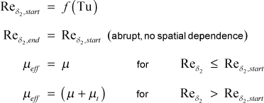
Abrupt Transition Model - For this transition model, the start and end Reynolds numbers are the same. This form of transition is often encountered when the flow encounters a surface disturbance such as roughness elements or boundary layer trip devices. A lower critical Reynolds number still applies, below which the flow will remain laminar, but the momentum deficit created by large surface disturbances usually increases the Reynolds number such that there is an abrupt transition to turbulent flow. For abrupt transition

For this model the momentum Reynolds number is introduced using the input variable gxx. Typical values for momentum Reynolds numbers at the start of transition range from 250-400 for Tu low, down to 150-200 for Tu>4%.

Intermittency Transition Model - The formulation of the intermittency model in the Prandtl mixing length model is
where γ is the intermittency function. In the models described here there is no y dependence for any of the intermittency functions.

Implementation of an intermittency model of transition is quite straightforward. There exists several variations in the open literature, but the basic model follows Abu-Ghannam and Shah¹, later refined by Mayle². In both models there is a function that defines the momentum thickness Reynolds number for the start of transition, and at that location, the -Reynolds number becomes Re_x,start .

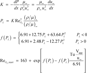
For the Abu-Ghannam and Shah model, the starting momentum Reynolds number is a function of both the local turbulence intensity and the local pressure gradient. For this model the turbulence intensity (Tu) is required to be in percent, and it is introduced using the input variable tuapp.

If k9>0, the transition starting correlation will be replaced by a specified starting momentum Reynolds number using the input variable gxx. This is designed primarily for flow over highly rough surfaces.

The end of transition, Re_x,end , can then be calculated using

The Abu-Ghannam and Shah intermittency function is

In summary,

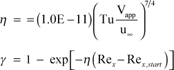
For the Mayle model, the starting momentum Reynolds number is only a function of the local turbulence intensity. For this model the turbulence intensity (Tu) is required to be in percent, and it is introduced using the input variable tuapp.

If k9>0, the transition starting correlation will be replaced by a specified starting momentum Reynolds number using the input variable gxx. This is designed primarily for flow over highly rough surfaces.

The Mayle intermittency function is
With the Mayle model, transition proceeds until γ>0.99 and beyond that point γ=1 and transition is considered finished.

Modified van Driest Transition Model - In this transition model, the van Driest damping function constant in the mixing length is controlled to simulate how the sublayer thickness decreases as the flow moves from a disturbed laminar flow into a fully turbulent flow, again for bypass levels of transition.

As with the intermittency models, the momentum thickness Reynolds number is used to identify the start of transition. Unlike traditional intermittency models, this starting momentum Reynolds number for transition is an input variable gxx, although it could be correlated in a manner similar to those used for intermittency models.

When transition begins, the van Driest damping function constant is set to the model constant C₁ and that value is continuously reduced using a sine function until the momentum Reynolds number reaches to a value equal to C₂ times the starting value of the Reynolds number
The effective van Driest damping function term (A_eff⁺) on the right hand side of the equation is the fully turbulent value computed as described in the mixing length model section. The recommended values for the constants are C1=1000 and C2=3.

Two-Equation Transition Model - This model is specific to the Lam-Bremhorst two-equation turbulence model and it was developed and documented by Schmidt and Patankar⁴. The model works with the k-equation by controlling the both the magnitude and rate of change of the P_k term

The model sets P_k=0 until the momentum thickness Reynolds number exceeds a certain value, introduced using the input variable axx. A nominal value for axx is 125. Therefore it is important that the starting x-Reynolds number is less than 1000 to insure the initial momentum Reynolds number is much less than axx. Transition predictions were extensively tested by Schmidt and shown to be mostly insensitive to the starting location providing the x-Reynolds number is small enough. Once the momentum Reynolds number exceeds axx the Schmidt production term modification (PTM) model is used to control the upper limit of the rate of change of the P_k term. The value of P_k at the integration location (x + Δx) is computed in a two-step procedure. First the P_k term is evaluated at the new x-location, and then the difference between its potential value and its value at the previous integration step is computed

Second, a PTM rate of change equation
is integrated to determine an upper limit to the change that will be permitted for P_k

The nondimensional constants in the model are computed using
and
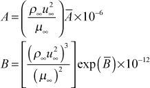
where Tu=(√k/u_∞). The constants are converted to dimensional constants using

The actual model constants A and B do not need to be computed every integration step, and intervals of 10 steps are sufficient because of the slow change in free stream velocity for typical integration stepsizes.

References

- 1
- Abu-Ghannam, B. J., and R. Shah, "Natural Transition of Boundary Layers - the Effects of Turbulence, Pressure Gradient, and Flow History," J. Mech. Eng. Sci., 22, 213, 1980.
- 2
- Mayle, R. E., "The Role of Laminar-Turbulent Transition in Gas Turbine Engines," J. Turbomachinery, 113, 509, 1991.
- 3
- Crawford, M. E., and W. M. Kays, STAN5 - A Program for Numerical Computation of Two-Dimensional Internal and External Boundary Layer Flows, NASA CR-2742, 1976.
- 4
- Schmidt, R. C., and S. V. Patankar, "Simulating Boundary Layer Transition With Low-Reynolds Number k-ε Turbulence Models: Part 2 - An Approach to Improving the Predictions," J. Turbomachinery, 113, 18, 1991.
- 5
- Mansour, N. N., J. Kim, and P. Moin, "Near-Wall k-ε Modeling," AIAA J., 27, 1068, 1989.
- 6
- Van Fossen, G. J., R. J. Simoneau, and C. Y. Ching, "The Influence of Turbulence Parameters, Reynolds Number and Body Shape on Stagnation Region Heat Transfer," J. Heat Transfer, 117, 597, 1995.
website updated Sept 2010 © 1996-2010 Michael E. Crawford - all rights reserved - website validated for CSS 2.1 and XHTML 1.0 strict at www.w3.org