one-equation model

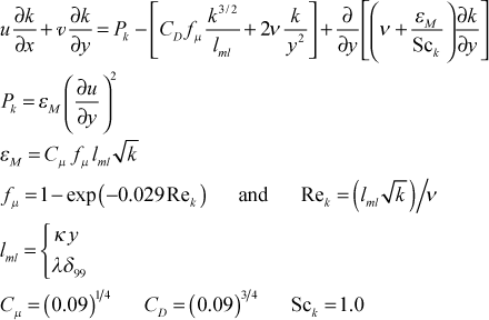
Summary - The one-equation formulation in TEXSTAN is

The flag ktmu identifies the one-equation model for computing the turbulent viscosity.

ktmu	one-equation turbulence kinetic energy model choice for external flows
= 11	Hassid-Poreh

Details - The one-equation turbulence-kinetic-energy can be used with the mixing length model, which provides the length scale for the model, and the model is really only suitable for boundary layer flows as it is currently programmed. It is an extension of what is described in Chap. 11 of CHMT and additional documentation can be found in Dawes¹, Hassid and Poreh², and Birch³, with the primary source being Hassid and Poreh. Because the one-equation model uses the mixing length, it is adaptable to the curvature model as well as the roughness model. A primary advantage of this model is that it can incorporate the effects of the free-stream turbulence via the outer boundary condition for the k-equation.

The boundary layer form of the transport equation for k, neglecting fluctuating body force work, is
where k is the arithmetic average of the three fluctuation components of velocity,
The transport equation is valid for flows away from a no-slip surface, where the flow tends to be isotropic, i.e. all three fluctuating components are similar in magnitude. For this formulation of the k-equation, the corresponding isotropic turbulence dissipation is given by
The isotropic turbulence dissipation term comes from combining the gradient of the fluctuating velocity-fluctuating viscous stress correlation, which represents the rate of work by the fluctuating viscous stresses of the turbulent flow, with the true dissipation, which is the fluctuating viscous stress tensor-fluctuating velocity-gradient correlation. Manipulation of these two terms leads to the isotropic term, ε, and the molecular term of the gradient transport term.

The Reynolds stress term is directly modeled using mean field closure, and the last two turbulent flow correlations in the gradient-diffusion term, transfer of k due to the turbulence itself and due to pressure fluctuations, are modeled using mean field closure and a turbulent diffusivity for k,

The final modeled transport equation for k becomes

We formulate the eddy diffusivity for momentum using dimensional analysis arguments and analogy to the Prandtl formulation
This shows the eddy diffusivity for momentum can be considered proportional to a length scale and a velocity scale that represent the turbulence behavior. Using this idea the one-equation formulation becomes

Here the length scale can be interpreted as a scale associated with the average size of the turbulent eddies, √ k represents the average turbulence velocity scale, and a is the model constant.

The model for the dissipation is also developed by analogy, and the guidance comes from evaluating the k-transport equation at the limits of the no-slip wall and the free stream.

For the free stream, the k-equation reduces to
which leads to the idea that at high Reynolds numbers (far from a wall) ε can be formed purely from velocity and length scales. From this dimensional insight we construct a model for ε that only uses these scales
where l_ε is the dissipation length scale.

We now consider the near-wall region where the x-convection is negligible and diffusion is also considered negligible (both assumptions confirmed by experimental measurements), called the Couette flow region. The momentum equation is reduced to

From conservation of mass and the Couette flow approximation, v=v_s. We now substitute
and the momentum equation reduces to
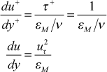
or in wall coordinates,
where y⁺ is the nondimensional distance from the wall in wall coordinates; u_τ is the shear velocity or friction velocity, u⁺ is the nondimensional velocity in wall coordinates, p⁺ is the nondimensional pressure gradient parameter in wall coordinates; v_s⁺ is the nondimensional wall transpiration parameter in wall coordinates; and τ⁺ is the nondimensional shear stress. The resulting ordinary differential equation integrates to the well-known Couette flow relationship

In the absence of pressure gradient and wall mass transpiration effects, this region is a constant total shear stress region. Recall that the mean field closure model for the total stress was

This model is recast into wall coordinates

The Couette flow region where ε_M>>ν is now examined. This is often called the log region where u⁺ is proportional to the natural log of y⁺. The total shear stress equation combines with the Couette flow equation to give or

With this formulation we now examine the k-equation in the Couette-flow region and we reduce it to two terms: production of k and dissipation of k, leading to the idea of production equals dissipation, or

Combining these two results leads to
where k⁺ is the nondimensional turbulence kinetic energy in wall coordinates. At this point it is generally assumed that the length scales for production and dissipation are similar and the ratio of length scales is removed,

Experimental information shows that k⁺ in this constant turbulent shear stress region is about 3 (we use 3.33, and it can range from 3-5) and we absorb a into C_D and we find C_D ≈ 0.09.

We now apply the mixing-length model, and we find the relationship between the dissipation length scale and the mixing length

Finally we make the assumption that the length scales for the production of k and the dissipation of k are nearly the same, and we establish the relationship between the mixing length and the length scale for k

With this relationship
and

The final model addresses the turbulent diffusion of k, where we use an idea similar to the turbulent Prandtl number for heat transfer,
We find that Sc_k=1.0 is a reasonable model constant.

To summarize, the eddy diffusivity for momentum becomes
or in terms of the turbulent viscosity,

The mixing length model was basically a two-scale model where l_ml is proportional to y in the near-wall region where the flow is extremely anisotropic and v^′ dominates, and l_ml is approximately constant in the high Reynolds number part of the flow where the flow is nominally isotropic.

This high-Re form of the k equation can be used in a hybrid or two-layer turbulence model that uses the mixing length formulation of the turbulent viscosity for the near wall region and the high-Reynolds number form of the one-equation model beyond about y⁺=100. This hybrid or two-layer model is often used in Navier-Stokes solutions (or so-called CFD solutions) because it avoids the need to compute in the near-wall region where the heat transfer modeling is very difficult, and the wall friction results are not so important for fluid mechanics results.

Because the k equation is valid only for high-Re turbulence, the equation needs to be modified to be able to compute it into the wall region. In this region the character of the turbulence changes and becomes strongly anisotropic. The √ k no longer really represents the average velocity scale (actually the v-component of k is more correct), and l=κy no longer represents the average length scale. We have seen this already in the mixing length model where the van Driest damping function needed to be added to correct the length scale. We first examine the dissipation term. At the wall
and from experimental measurements, k=y² in the region of the wall, leading to an idea of how ε behaves in the limit of the wall,
and it has a natural damping behavior for large y, where k asymptotes out to a constant value in the fully turbulent region. Thus we replace ε as the dissipation in the k-equation to include this low-Re wall term

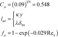
A second low-Re modification is to the length scale. In the mixing length we used the van Driest damping function to model the near wall behavior, especially in the sublayer, and we adopt a similar function for the one-equation model. For one- and two-equation models, it is customary to have this function multiply the length scale over the entire flow rather than have it applied only to the near-wall length scale (recall l_ml = κyD and l_ml = λδ, but it really makes no difference because the one-equation damping term asymptotically approaches unity at about the same location that the mixing-length damping function D approaches unity. The final form of the turbulent viscosity applicable to low-Re turbulence as well as high-Re turbulence is
where

Here the turbulence Reynolds number Re_k is based on the l_ml and √ k, and the damping constant value is suggested from the literature. To see the magnitude of this constant, convert the terms in the turbulence Reynolds number to wall coordinates and evaluate the Reynolds number in the fully turbulent part of the log region, y⁺=100 where k⁺ ≈ 3, leading to

We see the constant mostly damps out the f_μ effect (within 10%) by y⁺=100. Note that the f_μ damping function has a y² behavior in the limit as y goes to zero, giving an overall y⁴ damping of the turbulent viscosity as y goes to zero.

We need a low-Re modification to the isotropic part of the dissipation to remove it in the limit as y goes to zero. We adopt the same f_μ damping function so that the isotropic term is proportional to y⁴, matching the 4th power dependence of the production in the near-wall region where production balances dissipation (again the wall term naturally damps itself out)

Boundary Conditions - The boundary condition on k at the outer edge of the boundary layer comes from measurement of the flow-direction fluctuation in free stream velocity (u_∞), which is normalized and called flow-direction turbulence intensity,
and then converted to turbulence kinetic energy with the assumption that the fluctuations are isotropic, namely the same in all three coordinate directions. With this assumption the free stream turbulence kinetic energy becomes
where V_app is the approach velocity and Tu is the turbulence level at that same location. Values for Tu are traditionally reported in percentage, and it can range from so-called "low" values near 1%, associated with "quiet" experimental wind-tunnel facilities, and upwards to 20% or more associated with products of combustion. Tu can either be treated as frozen, that is, unchanging, or it is permitted to change in the flow direction, following the physics of the turbulence decay process.

References

- 1
- Dawes, W. N., "A Comparison of Zero and One Equation Turbulence Modeling for Turbomachinery Calculations," ASME Paper Number 90-GT-303, 1990.
- 2
- Hassid, S., and M. Poreh, "A Turbulent Energy Model for Flows with Drag Reduction," J. Fluids Engineering, 97, 234, 1975.
- 3
- Birch, N. T., "Navier-Stokes Predictions of Transition, Loss and Heat Transfer in a Turbine Cascade," ASME Paper Number 87-GT-22, 1987.
website updated Sept 2010 © 1996-2010 Michael E. Crawford - all rights reserved - website validated for CSS 2.1 and XHTML 1.0 strict at www.w3.org