two-equation model

Summary - For both internal and external flows, academic TEXSTAN code has a choice of 4 two-equation k-ε models by Launder and Sharma¹, Chien², Lam-Bremhorst, as described by Schmidt and Patankar³, and Jones-Launder⁴. These models vary in subtle details, and one of the constants in the Jones-Launder model is changed from the literature citation to permit better agreement with benchmark test cases. All other constants and functionals agree with the citations. The low-Re form of the k-ε equation set are

We formulate the eddy diffusivity for momentum similarly to what we did for the one-equation model, and we modify it for low-Re turbulence. We keep √k as the turbulence velocity scale and from dimensional analysis we form a turbulence length scale as l_t = (k^3/2/ε) and the eddy diffusivity for momentum becomes
or in terms of the turbulent viscosity, modified for low-Re turbulence

The flag ktmu identifies the four two-equation model choices for computing the turbulent viscosity.

ktmu	two-equation turbulence kinetic energy-energy dissipation model choices for internal and external flows
= 21	Launder-Sharma
= 22	KY Chien
= 23	Lam-Bremhorst
= 24	Jones-Launder

Details - The modeled high-Re transport equation for k is developed in the one-equation model section.

For the two-equation class, a high-Re transport equation for ε is developed and solved along with the k-equation, where the dissipation is defined the same as it was for the one-equation model

We can see the similarity in construction to the k-equation. The first term on the right of the equal sign is a production of dissipation, in analogy to the first term for the k-equation which is the production of k term. The second term is called the dissipation of dissipation, a term that causes destruction (or lowering) of ε, in exact analogy to how ε in the k-equation destroys (or lowers) the k value. The gradient terms are also similar. The turbulent part of the gradient term follows the nomenclature of Mansour, Kim, and Moin⁵ where the first term represents ε transfer due to the turbulence itself and the second term represents transfer due to pressure fluctuations, and the model uses mean field closure and a turbulent diffusivity for ε.

The models for the turbulent diffusion of k and ε use ideas similar to the turbulent Prandtl number for heat transfer,

We can rewrite both the k and ε equations into a more familiar form

In this formulation it is easy to see the (production - dissipation) term, and the inverse of the (k/ε) term in the ε equation has dimensions of time, and is often called the turbulent time scale term

We now reformulate the high-Re version of the k-ε equation set to permit calculations in the near-wall region where the turbulence becomes highly anisotropic. The dissipation term in the k equation follows that which was developed for the low-Re version of the one-equation model, where
and where the ε_wall term is often called the D term for two-equation models. Another modification is to add a source term to the epsilon equation to control the growth of the turbulent length scale (related to epsilon) and/or provide correct near-wall viscous sublayer behavior. This term is often called the E term. Additionally, functionals are added to the other source and sink terms of the epsilon equation.

The resulting low-Re form of the k-ε equation set become

We formulate the eddy diffusivity for momentum similarly to what we did for the one-equation model, and we modify it for low-Re turbulence. We keep √k as the turbulence velocity scale and from dimensional analysis we form a turbulence length scale as l_t = (k^3/2/ε) and the eddy diffusivity for momentum becomes
or in terms of the turbulent viscosity, modified for low-Re turbulence

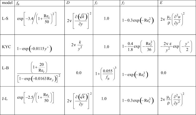
At this point the differences among the various two-equation turbulence models will depend on the set of constants and functionals, along with the appropriate epsilon wall boundary condition.
where
and the model constants are

We see that C_μ = 0.09, whereas for the one-equation C_D ≈ 0.09 and C_μ = (0.09)^1/4 = 0.548. To see why these are different, we recall the analysis leading to these coefficients, production equals dissipation which gave
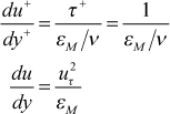
and in the Couette flow region where ε_M>>ν (the log region), the total shear stress equation combined with the Couette flow equation to give or

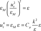
Combining these results for the two-equation model leads to or

Once again we use the same experimental information that k⁺ in this constant turbulent shear stress region is about 3 (we use 3.33, and it can range from 3-5), we find C_μ = 0.09.

We also comment on the dissipation equation constant C₂ (similar to the C_D coefficient for the one-equation model). When we consider how the k- and ε-equation behave in the free stream (the irrotational region beyond the edge of the boundary layer),

If we observe how k behaves for its decay behind grid-generated turbulence for a constant velocity and irrotational flow field, we see that ε can not be constant but must increase. Otherwise k would be unchanging (frozen). Using dimensional analysis ideas, we are lead to the form for the decay

This model works well to predict grid-generated turbulence decay with a value of C₂ ≈ 1.8-2.0 and this value changes somewhat with distance as the turbulence decays and becomes "weak".

Boundary Conditions - The ε wall boundary condition for the Launder-Sharma, K Y Chien, and Jones-Launder models is ε=0. For the Lam-Bremhorst model, the gradient of ε is set to zero, partly relating to how they developed their functionals and the fact that they do not need the D term.

For the k equation, the no-slip leads to k=0 at the wall, and for all the models the free stream boundary conditions are the same.

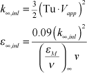
The boundary condition on k at the outer edge of the boundary layer comes from measurement of the flow-direction fluctuation in u_∞ , which is normalized and called flow-direction turbulence intensity, and then converted to turbulence kinetic energy with the assumption that the fluctuations are isotropic, namely the same in all three coordinate directions. With this assumption the free stream turbulence kinetic energy becomes
where V_app is the approach velocity and Tu is the turbulence level at that same location.

The free-stream boundary condition on the ε equation is typically set equal to (k_∞^1.5/L_e), where L_e is the local free-stream turbulence length scale at the location where Tu is measured. Several choices exist for the L_e scale. The most appropriate is the streamwise integral length scale obtained from the streamwise velocity autocorrelation. Note this should be about twice the vertical spatial scale if the flow is nearly isotropic. A second choice is the dissipation length scale, which relies heavily on the flow being homogeneous and isotropic. The dissipation scale is typically a factor of 2-3 larger than the integral scale. A third choice is to compute the length scale from a correlation if the turbulence was produced using a standard grid-generation scheme, similar to the procedure described by Van Fossen, Simoneau, and Ching, C. Y⁶. Whatever the choice, the resulting free stream ε should be on the order of 100 to 10,000.

For the two-equation models in TEXSTAN the initial free stream values are permitted to change by solving their transport equations, evaluated at the free stream. These are a set of ordinary differential equations
with the initial value of k coming from information on Tu and V_app (both input variables, tuapp and vapp) described above.

Note that these equations show that if you have an experimental distribution of free-stream k versus x, you can iteratively select the initial value of ε and solve this system of equations until the initial value matches the experimentally-measured decay rate for k.

If the input variable epsapp is set =0, the initial value for epsilon defaults to a TEXSTAN-calculated value from the two-equation definition of eddy diffusivity for momentum,

The model constant in this set of initial conditions is (ε_M /ν)_∞ and TEXSTAN uses (ε_M /ν)_∞ = 1000. For example, if the approach velocity is 50 m/s and the approach Tu is 5%, then for air, the approach k is about 9 m²/s² and the approach ε is about 400 m²/s³, and this value would reduce to about 80 m²/s³ if the approach velocity is 150 m/s. Both values are nominally within the order of magnitude range that was suggested. Note that if the user selects epsapp=0.01, it effectively freezes k_∞ .

References

- 1
- Launder, B. E., and B. I. Sharma, "Application of the Energy-Dissipation Model of Turbulence to the Calculation of Flow Near a Spinning Disc," Letters in Heat and Mass Transfer, 1, 131, 1974.
- 2
- Chien, K-Y, "Prediction of Channel and Boundary-Layer Flows With a Low-Reynolds-Number Turbulence Model," AIAA J., 20, 33, 1982.
- 3
- Schmidt, R. C., and S. V. Patankar, "Simulating Boundary Layer Transition With Low-Reynolds Numberk-ε Turbulence Models: Part 2 - An Approach to Improving the Predictions," J. of Turbomachinery, 113, 18, 1991.
- 4
- Jones, W. P., and B. E. Launder, "The Calculation of Low-Reynolds-Number Phenomena With a Two-Equation Model of Turbulence," Int. J. Heat Mass Transfer, 16, 1119, 1973.
- 5
- Mansour, N. N., J. Kim, and P. Moin, "Near-Wall k-ε Modeling," AIAA J., 27, 1068, 1989.
- 6
- Van Fossen, G. J., R. J. Simoneau, and C. Y. Ching, "The Influence of Turbulence Parameters, Reynolds Number and Body Shape on Stagnation Region Heat Transfer," J. Heat Transfer, 117, 597, 1995.
website updated Sept 2010 © 1996-2010 Michael E. Crawford - all rights reserved - website validated for CSS 2.1 and XHTML 1.0 strict at www.w3.org