initial profiles

Initial profiles are used to start the integration in TEXSTAN, and they can either be auto-generated using analytic equations programmed into TEXSTAN or they can be user-supplied profiles, typically from experimental data.

Auto-Generated Profiles - The auto-generated profiles for external flows use analytical equations that are programmed into TEXSTAN. The two choices are

• laminar or transitional flow profiles (kstart = 4,5,6,7)
• turbulent flow profiles (kstart = 3)

The laminar profiles are basically the Falkner-Skan profiles applicable to flow over a flat plate (Blasius, m=0), and flow in a 2-D stagnation region (m=1), applicable to 2-D stagnation-point flow, flow over a cylinder, or flow at the leading edge region of a turbine blade or vane. The laminar profiles serve to start transitional flows. The turbulent profile formulation uses the classic law-of-the-wall for the inner region and a power-law formulation for the outer region of the turbulent boundary layer. Both the turbulent profile generator and the laminar profile generator can provide initial profiles of the turbulence variables (turbulence kinetic energy and turbulence dissipation.

There are a set of six variables that describe the auto-generated profiles for any external flow. The variables dyi and rate set the y spacing for the velocity profile, which in turn controls the grid (finite difference mesh) for TEXSTAN. These variables have had considerable testing to establish values that yield grid-independent solutions (with respect to the cross-flow direction), and their recommended values are quite reliable. The variable tstag establishes the free stream temperature if the flow is constant properties, and the free stream stagnation temperature if the flow is variable properties. Note that if the energy equation is being solved, a temperature profile is always first constructed and then converted to a stagnation enthalpy profile if the flow is variable properties. The remaining three variables vapp and tuapp and epsapp are applicable only to transitional and fully-turbulent flows to describe the approach velocity and the approach turbulence intensity and turbulence dissipation.

Laminar or Transitional Flow Auto-Generated Profiles - This option is used primarily for laminar or transitional boundary layer flows over flat surfaces (kgeom=1) or over axisymmetric geometries (kgeom=2) or within axisymmetric geometries (kgeom=3). The option generates laminar velocity and other dependent variable profiles using the Falkner-Skan boundary layer theory. If a temperature profile is generated, it is based on a constant wall temperature boundary condition. If a mass transfer profile is generated, it is based on the momentum-mass transfer analogy and the value of the Schmidt number.

variable	value	description
dyi	5.0E-05
rate	0.09
tstag	= 0.0	only momentum equation being solved (neq=1)
	T∞	free stream static temperature (kfluid=1)
	T∞*	free stream stagnation temperature (kfluid>1)
vapp	= 0.0	flow never becomes turbulent (ktmu=0)
	= 0.0	transitional mixing length model
	Vapp	transitional 1- and 2-eqn models - approach velocity for computing kinl from Tu
tuapp	= 0.0	flow never becomes turbulent (ktmu=0)
	= 0.0	transitional mixing length model
	Tu	transitional 1- and 2-eqn models - Tu (in percent) for computing kinl
epsapp	= 0.0	flow never becomes turbulent (ktmu=0)
	= 0.0	transitional mixing length and 1-eqn models
	εinl	transitional 2-eqn model - initial value of turbulence dissipation
	=0.0	transitional 2-eqn model - TEXSTAN estimates initial value of turbulence dissipation

The variables dyi and rate set the y spacing for the velocity profile, where y is measured from the surface. The first y location in the grid is y(1)=0, and the second y location is calculated to be y(2))=del99*dyi, where del99 is the 99% boundary layer thickness, found by analyzing the velocity profile that is generated from the Falkner-Skan boundary layer theory. The next location is power-law expanded (sometimes referred to as a compound interest formulation) to be y(3)=y(2))*(1+rate), and so forth. The expansion is permitted to continue until the value of y exceeds 0.035*del99, and from that location outward, all y values are equally spaced at 0.035*del99. With this overall algorithm, there will be a significant number of points near the no-slip surface, depending on the values of both variables. For laminar flow, the suggested variables have been proven to provide grid-independent solutions over the laminar Re range. For transitional flow, the grid will be much finer to insure that once the flow becomes fully turbulent, there will be a significant number of points within the laminar sublayer (y⁺ ≤ 10 for smooth wall turbulent flows). Again the recommended values for dyi and rate have been tested for grid independent friction and heat transfer results.

To determine the velocity profile we use the Falkner-Skan boundary layer theory for the similarity solutions to the class of free stream velocity where u_∞ = Cx^m and
and the corresponding pressure gradient for the boundary layer flow is

The incompressible and constant property form of the boundary layer momentum equation is transformed using the Falkner-Skan transformation, formulated as
where the variable definitions and boundary conditions are given by

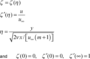
The Falkner-Skan equation is solved using a Runge-Kutta method, which requires ζ"(0). TEXSTAN has programmed into it curve fits for the values of the second derivative for m=0 (the Blasius equation where the free stream velocity is constant) and for m=1 (the two-dimensional stagnation point solution), which eliminates the need for an iterative method such as a shooting technique, but it restricts the solutions to m=0,1. These curve fits are valid for Prandtl number in the range 0.6 - 15, a wall-to-free stream temperature ratio of 0.99 - 1.01, and a Mach number less than about 0.05. The programmed solution can be used with either constant or variable properties, but it requires a constant wall temperature boundary condition. The user can violate these criteria, and although the initial profiles will not be correct, TEXSTAN will usually rapidly adjust.

The equation is solved over the range 0 < ζ < 7.5 to insure the profile extends well past the 99-percent boundary layer thickness location. For m=1, the 99-percent location will be much smaller than for m=0. From the Falkner-Skan solution the velocity profile is constructed and then the profile is evaluated to find del99. The profile is then interpolated at the mesh-generated y values using spline interpolation of the Falkner-Skan solution.

To determine the temperature profile we use corresponding Falkner-Skan constant property energy equation with no viscous dissipation is given by
where the Illingworth transformation is used and the variable definitions and boundary conditions are given by

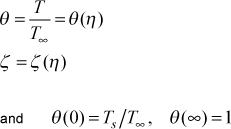
Note, for compressible flow, the stagnation temperature is used in place of the static temperature. When the heat transfer is required this equation is solved coupled with the Falkner-Skan momentum equation using a Runge-Kutta method. As with the momentum solution, the energy equation requires θ'(0) to avoid using the iterative shooting technique. TEXSTAN has programmed into it the values of the first derivative for Pr values corresponding to gases and light liquids for m=0 and for m=1. The profile is then interpolated at the mesh-generated y values using spline interpolation of the Falkner-Skan solution. Note that if the profile is for a variable property solution, the T(y) values are converted into stagnation enthalpy values at the y locations.

To determine the mass concentration profile we scale the Falkner-Skan velocity profile using the following ideas. We first equate the nondimensional velocity profile to the nondimensional concentration profile for each Falkner-Skan solution location
where m_j=(ρ_j /ρ_mix) is the mass concentration of component j, in units of kg(j)/kg(mix) or lbm(j)/lbm(mix), and solve for m_j(y). Then, scale the y location for momentum to the y location for this concentration value using

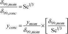
The profile is then interpolated at the mesh-generated y values using spline interpolation of m_j(y_conc).

To determine the turbulence kinetic energy and turbulence dissipation profiles, the initial values of k and ε at the edge of the boundary layer are first established. The edge value is k_inl,∞ is computed using the input variables tuapp and vapp and the definition

The edge value ε_inl,∞ is either an input variable (epsapp when epsapp > 0.001), or it is internally computed using a model based on the two-equation formulation of the turbulent viscosity

This formulation uses the two-equation C_μ = 0.09, and it requires a choice for the ratio of the turbulent to laminar viscosity ratio (ε_M / ν)_∞ at the edge of the turbulent boundary layer. This value is quite variable and it can be a function of the turbulence length scale in the free stream. It is estimated to be on the order of 100 - 1000, and TEXSTAN currently uses 1000.

The initial k profile is computed using the model

The initial ε profile is computed using the model
where

The behavior of this function is to reach a maximum in the near-wall region and then decrease towards zero. After ε(y) reaches a maximum and begins to decrease, it is constrained by requiring ε(y) > ε_inl,∞ . Note, for ktmu=23, the ε equation requires (∂ε/∂y) = 0, so the wall value of ε is set equal to its value at y(2). For all other ε equations, ε=0 at the wall.

Turbulent Flow Auto-Generated Profiles - This option is used primarily for turbulent external flows over flat surfaces (kgeom=1) to generate turbulent velocity and thermal profiles for a constant wall temperature boundary condition. The analytical development of these profiles is also used in the internal flows: initial profiles section of this website.

variable	value	description
dyi	0.1	interpreted as y+, wall coordinates
rate	0.175
tstag	= 0.0	only momentum equation being solved (neq=1)
	T∞	free stream static temperature (kfluid=1)
	T∞*	free stream stagnation temperature (kfluid>1)
vapp	= 0.0	mixing length model
	Vapp	1- and 2-eqn models - approach velocity for computing kinl from Tu
tuapp	= 0.0	mixing length model
	Tu	1- and 2-eqn models - Tu (in percent) for computing kinl
epsapp	= 0.0	mixing length and 1-eqn models
	εinl	2-eqn model - initial value of turbulence dissipation
	=0.0	2-eqn model - TEXSTAN estimates initial value of turbulence dissipation

The variables dyi and rate set the y spacing for the velocity profile, where y is measured from the surface. There definitions are completely different from those used for kstart=4 (laminar and transitional flows), but the overall procedure for computing the y-distribution remains qualitatively the same. For developing the grid with turbulent profiles, the grid is first established in wall or plus coordinates, and then converted to physical coordinates. The first y⁺ location in the grid is =0, and the second y⁺ location is calculated as y⁺(2)=dyi. The next location is power-law expanded (sometimes referred to as a compound interest formulation) to be y⁺(3)=y⁺(2)*(1+rate), and so forth. The expansion is permitted to continue until the value of y⁺ exceeds 0.035*δ₉₉⁺ and from that location outward, all y⁺ values are equally spaced at 0.035*δ₉₉⁺.

The variable δ₉₉⁺ = (δ₉₉)/(ν / u_τ) is the physical upper limit for y converted to plus coordinates, and del99 is the 99-percent boundary layer thickness. To calculate del99 = δ and u_τ = √(τ_wall/ρ) = u_∞ √(c_f /2), standard correlations for the flat plate turbulent boundary layer are used for the friction factor, c_f /2 = 0.0125 / (Re_δ2^0.25), and for the relationship between the momentum thickness and the boundary layer thickness (for a 1/7 power law approximation), (δ₂ / δ) = 0.097.

TEXSTAN develops the starting value of c_f /2 from the input variables that permit calculation of a starting x-Reynolds number, which is adjusted using a virtual origin to accurately control the starting momentum thickness Reynolds number. This is described in detail in the definition of the input variable k1.

With this overall algorithm, there will be a significant number of points near the no-slip surface, depending on the values of both variables. The recommended values for dyi and rate have been tested for grid independent friction and heat transfer results. Once the grid is established in plus coordinates, turbulent boundary layer theory and the mixing length turbulence model are used to obtain the velocity and temperature profiles.

To determine the velocity profile we divide the boundary layer into an inner layer and an outer layer. For the inner layer we determine the velocity using mean field closure, the Couette flow approximation to the total shear stress, and the mixing length turbulence model. For the outer layer we determine the velocity using the power-law form of the velocity law-of-the-wall.

For the inner layer mean field closure equation will become the calculating equation for how the velocity varies with y inside the boundary layer. The total shear stress in the turbulent boundary layer is composed of the molecular term and the Reynolds stress term
where the molecular term is modeled using Newton's law of viscosity and the turbulent term is modeled using mean field closure, leading to the mean field closure equation
and ν is the molecular momentum diffusivity and ε_M is the turbulent momentum diffusivity.

In plus coordinates this equation becomes
where the wall or plus coordinates are defined as follows

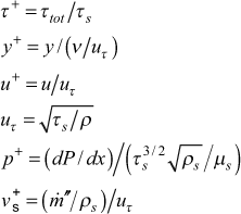
We now need a model for the total shear stress and a model for the turbulent (or eddy) viscosity. For the total shear stress the Couette flow assumption (neglecting dx-convection) leads to the total stress in plus coordinates given by
and the mean field closure model for calculating equation for the inner-layer velocity profile becomes

For the inner layer we use the mixing length formulation from the classical Prandtl model,
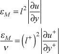
where the complete formulation of the mixing length is
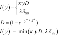
and l⁺ = l /(ν / u_τ). The model constants (or functionals) used in calculating the turbulent velocity profile are exactly the same as those described in detail in the modeling: mixing length model section of this website. When we combine these equations and we have
along with the Couette flow equation for τ⁺ . This equation is integrated until (κy⁺D) = (λδ⁺), and then the model smoothly changes into the outer layer power law model.

The outer layer model is the power-law formulation
where n is calculated by evaluating the function at the last value of u(y) from the inner layer calculation.

To determine the temperature profile we again divide the boundary layer into an inner layer and an outer layer. For the inner layer we determine the temperature using mean field closure, the Couette flow approximation to the total heat flux, and the combination of the mixing length turbulence model and the variable turbulent Prandtl number model. For the outer layer we determine the temperature using the power-law form of the thermal law-of-the-wall.

For the inner layer mean field closure equation will become the calculating equation for how the temperature varies with y inside the boundary layer. The total surface heat flux in the turbulent boundary layer is composed of the molecular term and the Reynolds stress term
where the molecular term is modeled using Fourier's law and the turbulent term is modeled using mean field closure, leading to the mean field closure equation
and α is the molecular thermal diffusivity and ε_H is the turbulent thermal diffusivity.

In plus coordinates this equation becomes
where

We now need a model for the total heat flux and a model for the turbulent (or eddy) conductivity. For the total heat flux the Couette flow assumption (neglecting x-convection) leads to the total stress in plus coordinates given by
(similar to the Couette flow form of the total shear stress), and the mean field closure model for calculating equation for the inner-layer temperature profile becomes
where the turbulent Prandtl number is Pr_t = (ε_M / ε_H) .

The model constants (or functionals) used in calculating the turbulent temperature profile are exactly the same as those described in detail in the modeling: mixing length model and the modeling: turbulent Prandtl number sections of this website, along with the Couette flow equation for q⁺ .

When the velocity model switches to its outer-layer model, the model for temperature smoothly changes into its outer layer power law model
where m is calculated by evaluating the function at the last value of T(y) from the inner layer calculation. In principal, we should use the thermal boundary layer thickness rather than the momentum boundary layer thickness, but there are enough approximations to make this not very useful for turbulent flow, unless liquids are being used (especially liquid metals). To obtain the surface heat flux, we use the Chilton-Colburn-Reynolds analogy to calculate the heat transfer coefficient, StPr^2/3 = c_f /2 , and the convective rate equation q_s" = h(T_s-T_∞).

To determine the turbulence kinetic energy profile we again divide the boundary layer into an inner layer and an outer layer. For the inner layer (assumed to coincide with the velocity inner layer) we determine the k using the one-equation model
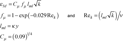
as described in the modeling: one equation model section of this website. We solve for k(y) using the ε_M value from the velocity profile calculation. Note this is iterative at each y) location because Re_k is a function of k.

For the outer layer there really is no theoretical basis, and instead we use a 3rd order polynomial curve fit between the beginning of the outer layer and the edge of the velocity boundary layer. Here again, we would realistically expect the edge of the k boundary layer to be larger than the velocity boundary layer, so this may be a significant approximation. For the 4 coefficients of the 3rd order polynomial we fit value and slope (derivative) at the inner-layer outer-layer point and at the edge of the boundary layer. The edge value is k_inl,∞, computed using the input turbulence level, tuapp (in percent) and the value of the free stream velocity at xstart,

To determine the turbulence dissipation profile we divide the boundary layer into an inner layer and an outer layer. For the inner layer (assumed to coincide with the velocity inner layer) we determine ε using the definition for the two-equation model,
and choose the C_μ and functional that matches the two-equation model (ktmu) that is being used. Note that some of the models will require iteration.

The outer layer is computed using the same idea used for the k profile outer layer. The edge value is ε_inl,∞, and it is either an input variable (epsapp when epsapp > 0.001), or it is internally computed using a model based on the two-equation formulation of the turbulent viscosity

This formulation uses the two-equation C_μ = 0.09, and it requires a choice for the ratio of the turbulent to laminar viscosity ratio (ε_M / ν)_∞ at the edge of the turbulent boundary layer. This value is quite variable and it can be a function of the turbulence length scale in the free stream. It is estimated to be on the order of 100 - 1000, and TEXSTAN currently uses 1000.

We close by discussing two-equation calculations, and we note that the resulting friction and heat transfer results are somewhat sensitive to the choice of the (ε_M / ν)_∞ value for determining ε_inl,∞. Furthermore, the initial profiles of k and ε are so approximate that the user will likely see somewhat unstable behavior in these variables (and the resulting friction and heat transfer) until the effect of the initial conditions are damped out, which sometimes takes a significant momentum Reynolds number flow length. This can potentially be a problem for highly accelerated flows where the momentum Reynolds number never really becomes large.

This is one reason we often use the k10=21-25 flag to print profiles for restarting TEXSTAN if we are studying the behaviors of turbulence models. The user can start the flow turbulent using kstart=3, and after the momentum Reynolds number has doubled, print profiles using the k10 flag. These profiles can then become the turbulent starting profiles (using kstart=0) rather than using kstart=3.

A second approach to obtaining turbulent starting profiles for two-equation models is to start the flow turbulent at a very low momentum Reynolds number (10-20) and let the two-equation model naturally transition (no model). The user can then use the k10 flag and choose a momentum Reynolds number that represents fully turbulent flow (1000-2000). At this Reynolds number the profiles become very stable starting profiles for k and ε that are self-consistent with the two-equation model being studied. We reiterate, the kstart=3 profiles are very simple approximations.

User-Supplied Profiles - The primary reason TEXSTAN has auto-generated profiles is that auto-generated profiles yield grid-independent solutions. When user-supplied profiles are chosen as a method to start TEXSTAN, the user may risk not achieving grid independence as described in the overview: numerical accuracy section of this website. The choices are

kstart	special user-supplied initial profile options
=0	primarily designed for restart of TEXSTAN based on a dump of profiles from a previous calculation
=10	primarily designed to input experimental profiles, selected kgeom and turbulence models

It is extremely important that the distribution of profile points in any input profile (TEXSTAN-generated or user-supplied) be correct. When kstart=0 is selected, the user provides the input profile with a guaranteed correct u(y) distribution, and when kstart=10, the user provides a set of u(y) data points (typically 15=20) from an analytical solution or from experimental data, and TEXSTAN interpolates the profile using the same algorithm for data point distribution that is used when TEXSTAN internally makes a set of initial profiles.

          Profiles for kstart=0 - This option should really only be used to restart TEXSTAN, and the profiles come from a previous TEXSTAN run. Restart profiles are generated by setting k10=21-25 as described in the profiles (velocity and temperature) - standard output part of external flows: output files section. Use of restart profiles is particularly helpful for the study of turbulence models.

For reference we begin by discussing what a TEXSTAN input dataset looks like if profiles are being generated within TEXSTAN (any kstart value except =0,10). Here is a partial listing from the s10.dat.txt benchmark case, showing the last four lines of the input data

The last data line contains the instructions for how TEXSTAN will create initial profiles. With kstart=0,10, you will be replacing these last two data lines.

When k10=21-25 is used along with bxx, two files are written: ftn73.txt and ftn74.txt. The file ftn73.txt contains the profile for restarting TEXSTAN, and it is correctly formatted to be easily used with kstart=0. Here is a partial listing of ftn73.txt. It was generated by running TEXSTAN using the s10.dat.txt benchmark dataset whose starting x-Reynolds =1000. Two variables were changed in s10.dat.txt to generated this ftn file. The variable k10 was set =22 and the variable bxx was set =50, (you could also use k10=21 and bxx=5700 in that dataset). When TEXSTAN is restarted using information from the ftn73.txt file, the integration will begin at a momentum thickness Reynolds number =50 and a corresponding x-Reynolds number =5700.

ftn73.txt - a partial listing
where the following TEXSTAN variables translate into physical variables

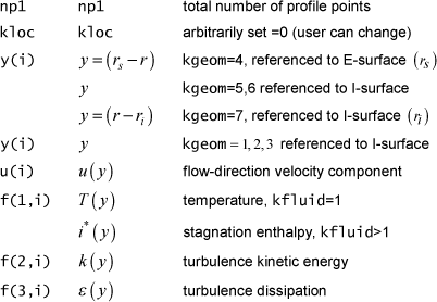
There are two ways to use the ftn73.txt file, depending on the choice of the kloc variable

kloc	flag for use with kstart=0, 10
=0	user places the TEXSTAN-generated restart profiles within the TEXSTAN input dataset
=1	user places the TEXSTAN-generated restart profiles in a separately named data file

To use kloc=0, the procedure to convert a TEXSTAN dataset is as follows

• (a) change kstart to =0
• (b) replace the last two data lines of the TEXSTAN dataset with the entire ftn73.txt file

Here is a partial listing that shows what the TEXSTAN input dataset looks like when kloc=0 is being used and the last two data lines are replaced by the entire ftn73.txt file. The listing comes from the t10n.dat.txt benchmark case.

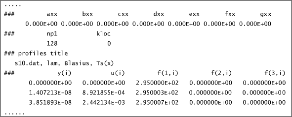
We recognize that all the data lines beyond the two data lines (### and axx, bxx, ..., gxx) are the contents of ftn73.txt.

To use kloc=1, the procedure to convert a TEXSTAN dataset involves changing the input data file and the ftn73.txt file. The changes to the input data file are

• (a) reset kstart =1
• (b) delete the last two data lines of the TEXSTAN dataset and replace them with a copy of the first four data lines of the ftn73.txt file
• (c) in the first copied data line reset kloc =1
• (d) in the fourth copied data line change the text to be the name of the file that will contain the profile (it is ok to call it ftn73.txt, or in the example we will use, it is called p10n.pro.txt

The changes to the ftn73.txt file are

• (e) remove the first 3 lines of the ftn73.txt file
• (f) rename the file ftn73.txt to whatever you choose (in this example it was renamed p10n.pro.txt)

Here is a partial listing that shows what the TEXSTAN input dataset looks like when kloc=1 is being used. The listing comes from the p10n.dat.txt benchmark case.

The modified ftn73.txt file is renamed p10n.pro.txt. Here is a partial listing of that file.

          Profiles for kstart=10 - This option is useful if the user plans to start TEXSTAN with experimental profiles or if no initial profiles are available, as is the case with free convection flows. The profiles are read and then their y-distribution is interpolated onto a much finer grid (finite difference mesh) that is created by TEXSTAN using the variables dyi and rate, and designed to ensure a grid-independent solution.

If the energy equation is being solved, it is assumed the user has supplied an initial temperature profile. Then, if variable properties are being considered, the temperature profile will be converted to a stagnation enthalpy profile within TEXSTAN.

If the user is working with turbulent flow and has an experimental turbulence kinetic energy initial profile but not the corresponding experimental dissipation profile, but intends to use a two-equation turbulence model with TEXSTAN, there is a provision to create a turbulence dissipation profile, using the same formulation as with the auto-generated dissipation profile. This choice is flagged using the epsapp variable.

To show an example of how kstart=10 is used, we take an initial profile (from a file called ftn73.txt), and we remove most of its points, leaving 17 points in the outer region of the flow. We recognize that this is much too thin a boundary layer for normal experimental measurement techniques, but it will serve to demonstrate the kstart=10 choice.

Here is a partial listing that shows what the TEXSTAN input dataset looks like when kloc=0. Note that we have added two lines at the end of the dataset to tell TEXSTAN how to interpolate the data to expand it into an acceptable y-distribution for the finite difference grid, and the dataset is renamed t10nn.txt. Here is a partial listing of the dataset.

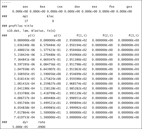
We recognize the last two data lines, which contain dyi and rate, described in the overview: numerical accuracy section of this website. These variables control the development of the grid (finite difference mesh) for TEXSTAN. These are used to construct a fine-meshed grid onto which the experimental or sparse velocity profile will be interpolated to create an expanded profile.

The initial velocity profile is first examined and the velocity boundary layer thickness (del99) is determined. Then the first y location away from the wall is calculated to be y(2)=del99*dyi. The next location is power-law expanded to be y(3)=y(2)*(1+rate), and so forth. The expansion is permitted to continue until the value of y = 0.035*del99, and at that location, all y values are equal spaced at 0.035*del99. This algorithm is used for both planar and axisymmetric coordinates, and then for kgeom=4,5, the coordinate is linearly transformed such that y=0 becomes the centerline. With this overall algorithm, there will be a significant number of points near the no-slip surface. Once the fine-mesh grid is established, the input set of profiles (velocity, temperature, and such) are interpolated onto the fine grid using a 3rd order spline, which insures a fine grid near the wall and that expands in a power-law away from the wall.

For kloc=1, here is a partial listing that shows what the modified s10.dat.txt input dataset looks like. Note the similarity to what was used for kstart=0 except that there are two data lines added after the profile data file name to set the dyi and rate values.

The dataset refers to the p10nn.pro.txt file. This data file is obtained by taking the p10n.pro.txt profile dataset and reducing it to 17 data points for use with kloc=0 and renaming it. Here is a partial listing of p10nn.pro.txt.