boundary condition smoothness

There are certain boundary condition arrays in TEXSTAN that demand smoothness, because the interpolated arrays are differentiated and the derivatives are used in the transport equations. These arrays include the velocity ubE(m) array, which is used to form the external flow pressure gradient, the wall radius rw(m) array for use in modeling of axisymmetric supersonic nozzles, and the aux3(m) array for use with the mixing length model when axial curvature is being considered.

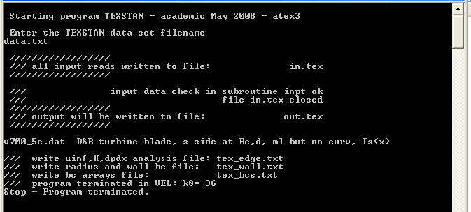
To determine if the boundary conditions are mathematically smooth, the user needs to modify the TEXSTAN input file using k8=36 and then run TEXSTAN using the input dataset. The benchmark dataset v700_5e.dat.txt, described in the section turbine blade, is used to demonstrate the concepts in boundary condition smoothness. The dataset is modified and renamed data.txt. TEXSTAN is then started, the dataset name is typed in, and execution begins.

After the dataset goes into execution, its free stream velocity array and the boundary condition array are analyzed, and the execution is stopped without proceeding to integrate. Three analysis files are generated:

• tex_edge.txt
• tex_wall.txt
• tex_bcs.txt

The first two files contain data that can be plotted to observe smoothness. The third file is not particularly useful and is not described here.

Free Stream Velocity Smoothness - The free stream velocity array, ubE(m), at each x(m) location is created from either a u_∞(x) function or from experimental data for edge velocity or Mach number. It is important that the ubI(m) array be mathematically very smooth, because it is interpolated and used to create the pressure gradient from Bernoulli's equation. The pressure gradient then becomes the source function in the momentum equation. TEXSTAN uses cubic spline interpolation of the free stream velocity to help create a smooth velocity gradient in forming the pressure gradient.

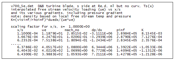
For external flows, the procedure in TEXSTAN to calculate the pressure gradient is to spline-fit free stream velocity array to provide a continuous u(x) distribution and to provide its derivative, du/dx, from which the pressure gradient (dp/dx) is constructed using a Bernoulli formulation. The free stream velocity smoothness analysis is basically evaluation of this pressure gradient procedure at 250 equally spaced intervals (x locations) over the interval xstart < = x <= xend, and the results are written into the tex_edge.txt file. As a part of the analysis, the pressure gradient is integrated to determine how the free stream static pressure distribution will vary with x, and the Mach number and K acceleration parameter distributions are computed as a function of x.

The following example is taken from the turbine blade benchmark dataset v700_5e.dat.txt. The analysis file is tex_edge.txt, and the following is a sample from this file:
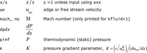
where

Plotting this pressure gradient distribution will help the user be sure their free stream velocity array, ubE(m), is differentially smooth. If it is not smooth, then some type of numerical smoothing software, perhaps using a least-squares method, needs to be used to smooth the array. Once the velocity array is smoothed, it needs to be rechecked for smoothness. Once again, it is imperative the pressure gradient distribution is smooth, especially for flow over turbine airfoils (blades and vanes), and the user can not be assured the pressure gradient is smooth by examination of the velocity profile by itself.

Wall Variable Smoothness - There are several other wall variables that need to be smooth. For axisymmetric flows (kgeom=2,3 for flow over missiles or spheres or inside axisymmetric nozzles) the wall transverse radius variable is contained in the rw(m) array. TEXSTAN uses the wall radius derivative, called csalfa, in the transformed governing equations. For heat transfer, the input wall boundary condition, either wall temperature for jbc(j)=1 or wall heat flux for jbc(j)=2, is contained in the energy equation's fj(I,j,m) array. For flows using the curvature-modified mixing length model, kgeom=1 and ktmu=5,11, the radius of curvature variable is contained in the aux3(m) array. All of these arrays should be considered for smoothing, especially if the boundary condition information is from experimental data.

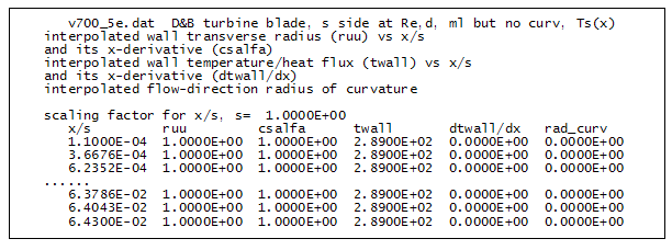
For the wall boundary condition analysis TEXSTAN takes the x distribution, xstart < = x <= xend and sub-divides it into 250 equally spaced intervals. The expanded wall arrays, including the first derivatives of the wall transverse radius and wall temperature, are then linearly interpolated, and the results are written into the tex_wall.txt file. The following example is taken from the turbine blade benchmark dataset v700_5e.dat.txt. The analysis file is tex_wall.txt, and the following is a sample from this file:
where

Plotting the csalfa distribution will help the user be sure transverse radius of curvature array, rw(m), is differentially smooth. There is currently no print-out of the derivative of the axial wall radius of curvature R primarily because in the curvature model only 1/R is used (no derivatives), and the model is not that sensitive to smoothness (see modeling: curvature section).