computational results

The Blasius problem supports CHMT problems 9.7 (for momentum) and 10.16 (for heat transfer). The problem assumptions include constant properties; neglect viscous dissipation, and laminar flow over the entire surface. The temperature ratio and Mach number (air as an ideal gas) for this problem are

• T_s / T_∞ = (295.0)/(300.0) = 0.98
• M = u_∞ /(γRT) ^0.5 = (15.0)/ [(1.4)(8314/28.97)(300)]^0.5 = 0.05

These calculations support the assumption of constant properties and the assumption that it is ok to ignore viscous dissipation. The trailing edge x-Reynolds number is 2 x 10⁵, which supports the assumption of laminar flow, and the fact that we do not need to consider transition.

Momentum Transfer Results - These computational results are compared with the analytical Blasius similarity solution.

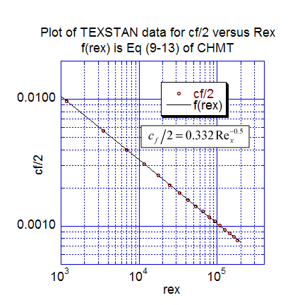
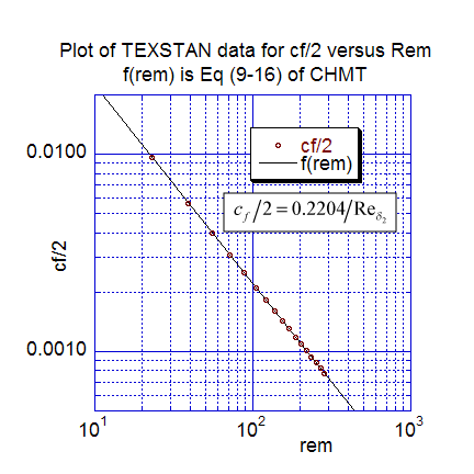
The first momentum transfer results present the local friction coefficient data distribution. The first plot is c_f/2 versus the x-Reynolds number, and the computations are compared with Eq. 9-13 of CHMT 4th ed. (note Eq. 9-13 was modified to c_f/2 rather than c_f to compare with the TEXSTAN output). The second plot is the local friction coefficient distribution replotted as a function of the momentum-thickness Reynolds number and compared with Eq. 9-16 (CHMT 4th ed.). The TEXSTAN results for these two plots are extracted from s10.ftn85.txt.

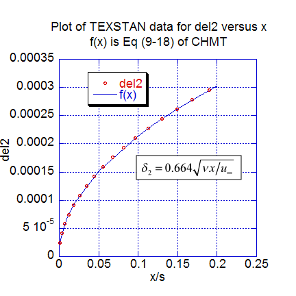
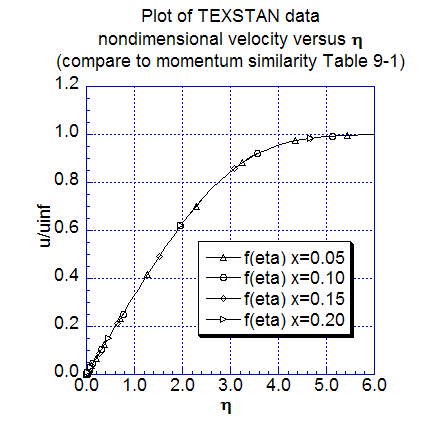
The next two figures show additional momentum transfer results. The local momentum thickness data distribution is plotted as a function of x, extracted from s10.ftn84.txt, and compared with Eq. 9-18 (CHMT 4th ed.). Velocity profiles, nondimensionalized using the Blasius variables are plotted for several nondimensional x locations. These profile results can be compared to Table 9-1 (CHMT 4th ed.) to demonstrate the characteristics of self-similar flow at different x-locations and to confirm the 99-percent velocity boundary layer thickness and its approximation, Eq. 9-33 (CHMT 4th ed.). Note the profiles were generated by resetting flag kout=2 and k10=10 in s10.dat.txt.

Heat Transfer Results - These computational results are compared with the analytical Blasius similarity solution.

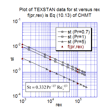
The first heat transfer results present nondimensional heat transfer in two traditional forms. The first plot is local Nusselt number data distribution versus the x-Reynolds number for three Prandtl numbers (0.7, 1, and 5), and the computations are compared with Eq. 10-10 (CHMT 4th ed.). The second plot is the local Stanton number distribution versus the x-Reynolds number for three Prandtl numbers (0.7, 1, and 5), and the computations are compared with Eq. 10-13 (CHMT 4th ed.). Of particular note in the Stanton number plot is the results for Pr=1, which is the classic Reynolds analogy test. Also, we could have plotted the data as St-Pr^2/3 and the data would have collapsed onto a single line, as suggested by Eq. 10-13. The TEXSTAN results for these two plots are extracted from s10.ftn85.txt.
note: the s10.dat.txt dataset can be used for either the Pr=0.7 or the Pr=1 case by simply changing the Pr value. To test this benchmark data set for water (Pr=5), data set needs several minor changes. The fluid properties of density, dynamic viscosity, specific heat need to be changed to match the properties of water, and the start and stop variables (xstart and xend) need to be changed to match the starting x-Reynolds number ~ 1000 and stopping x-Reynolds number ~ 2 x 10⁵ requirements.

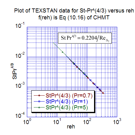
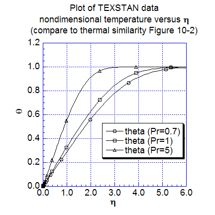
The next two figures show additional heat transfer results. The first plot is the local Stanton number distribution replotted as a function of the enthalpy-thickness Reynolds number for three Prandtl numbers (0.7, 1, and 5), and the computations are compared with Eq. 10-16 (CHMT 4th ed.). The TEXSTAN results for this plot are extracted from s10.ftn85.txt. Temperature profiles, nondimensionalized using the Blasius variables are plotted for several nondimensional x locations. These profile results can be compared to Figure 10-2 (CHMT 4th ed.) to demonstrate the characteristics of self-similar flow at different x-locations. To confirm the 99-percent thermal boundary layer thickness, one can calculate the ratio of the thermal boundary layer thickness to either the computational or theoretical momentum boundary layer thickness and compare the ratio to the approximation in Eq. 10-27 (CHMT 4th ed.). Note the profiles were generated by resetting flag kout=2 and k10=10 in s10.dat.txt.

At this time there are no graphics associated with TEXSTAN, although the output files are designed to permit importing into various graphical packages; these plots have been carried out using the superb, user-friendly plot package KaleidaGraph from Synergy Software.