computational results

The benchmark turbine blade flow occurs over the suction side of the airfoil with constant wall temperature and variable free stream velocity. The flow is a transitional boundary layer flow that remains attached from the stagnation point region to the blade trailing edge.

Velocity Boundary Condition - The free stream velocity array for this dataset was obtained from Daniels experimental data for the blade suction-side velocity distribution, with a total of 19 data points (nxbc(I)=19). When the v700_5e.dat.txt dataset was first constructed, the data was analyzed using the procedures outlined in the overview: bc smoothness section of this website. The results showed a tendency for an abnormal adverse pressure gradient near the leading edge after the initial region of strong acceleration, and while TEXSTAN did not stop due to flow separation, the artificial adverse pressure gradient can affect a mixing-length turbulence model that uses a pressure-gradient correction term. Note that two-equation turbulence models are not strongly affected by this pressure gradient anomaly.

A least-squares software was applied to the data to smooth the free stream velocity array, resulting in really only minor adjustments to the free stream velocity in the leading edge region. The smoothed free stream velocity profile is what is used in the current v700_5e.dat.txt dataset. TEXSTAN was tested with and without the smoothed free steam velocity array and the results were minimal in prediction of the surface heat transfer, presented in the Heat Transfer Results block. The benchmark dataset was modified by setting k8=36, and several data plots have been constructed using the resulting analysis file tex_edge.txt to show how the free stream velocity distribution behaves for this test case.

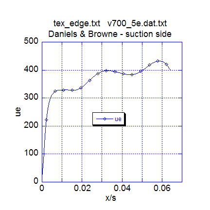
The first plot presents the smoothed free stream velocity distribution for the turbine blade. The plot shows a smoothly varying velocity distribution that begins at stagnation, accelerates over the initial part of the blade leading edge, then flattens out, followed by a milder acceleration, a slight deceleration, a mild acceleration, and then a deceleration near the trailing edge. This trailing edge behavior is to be expected because there is really no experimental data resolution in that region. Before the experimental velocity array was smoothed, the region near the leading edge where the acceleration goes to zero was incorrect. The TEXSTAN spline-fit to the original experimental velocity array showed a small region of sharp deceleration rather than the near-zero acceleration. Typically, the region beyond the initial strongly accelerating leading edge region is troublesome for boundary layer calculations, especially when the blade design is highly front-loaded. TEXSTAN generally will show a boundary layer separation, which causes the TEXSTAN code to fault and stop. Generally, there is no experimental evidence of this localized separation, and it is an artifact of either the experimental (or Euler-produced) data or due to how TEXSTAN spline-fits data. Always, it is troublesome to spline-fit sharply-changing data, but spline-fit routines are useful for producing continuous first derivatives of the data, necessary for the pressure gradient formulation.

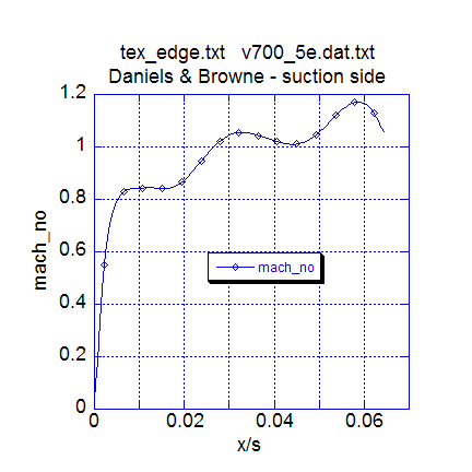
The second plot presents the turbine blade Mach number distribution. The experimental heat transfer data do not really reflect much of a numerical simulation problem for TEXSTAN, and this suggests the flow Reynolds number is low enough to minimize these effects. Note that there are no explicit shock-boundary layer mechanisms built into TEXSTAN.

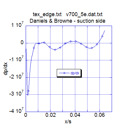
The third plot presents the resulting pressure gradient distribution. We see in the plot a reflection of how the free stream velocity accelerated and decelerated, and we can identify regions of zero pressure gradient, and overall the pressure gradient distribution is quite smooth. This plot is equally important to the free stream velocity distribution plot, because if the velocity array is not smooth, the pressure gradient will tend to be erratic, and possibly oscillate between positive and negative values. Again, this effect is mostly a problem for mixing-length turbulence models, and TEXSTAN has a damping function built into the mixing length pressure gradient parameter to attenuate the oscillatory effects (see the modeling: mixing length model section of this website for a description of the lag function that damps the model).

Heat Transfer Results - Verification of the variable properties assumption is two-fold: assessment of the flow Mach number and assessment of the temperature ratio (T_s / T_∞). Either effect can lead to strong variation in the thermophysical properties and a requirement to use variable properties (kfluid > 1) and viscous dissipation or viscous work (jsor =3) for the energy equation.

The Daniels and Browne turbine blade flow is highly compressible, as can be seen from the Mach number distribution over the blade, and this effect by itself leads to a variable property behavior due to near-wall viscous work. This can be verified by examining a thermal profile in the high-Mach number part of the blade. For this dataset, the flag k10=22 creates a set of profiles at the momentum thickness Reynolds number set by the specification of bxx (= 2000.0), which is about the x = 0.05 meters location on the blade surface. From output file ftn74.txt, the temperature at the free stream is 3.390887E+02 Kelvins, and the blade surface temperature is held constant at 289.0 Kelvins. Thus the ratio T_s / T_∞ = (289.0)/(339.0) = 0.85, a significant heating condition and requiring the variable property assumption.

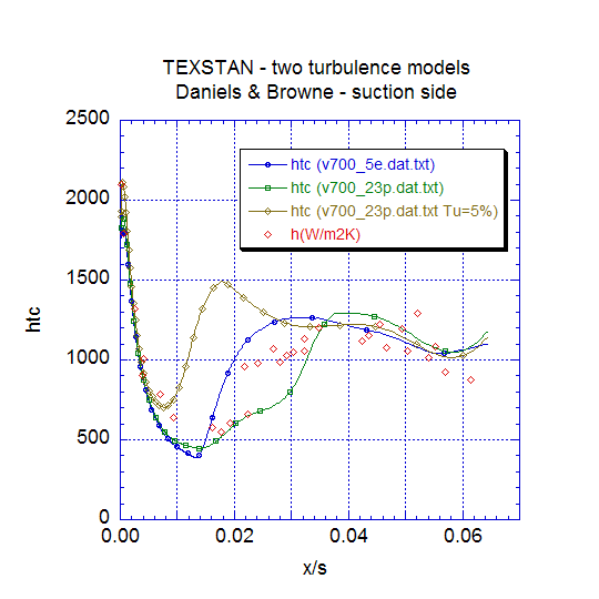
Verification of the Daniels and Browne benchmark dataset is primarily based on comparing the experimental heat transfer coefficient distribution with TEXSTAN. Two benchmark datasets have been used, the mixing-length model v700_5e.dat.txt and the two-equation Lam-Bremhorst model with controlled transition,v700_23p.dat.txt. With this two-equation dataset, the accepted value of tuapp =3.0 (in percent) and epsapp = 8231 m²/s³ were used. A variation was also tested where tuapp was set = 5.0 to demonstrate the effects of increase in free stream turbulence. Note that both of levels of free stream turbulence intensity (Tu) constitute bypass-level transition, where the normal transition structures that occur in low levels of free stream turbulence are missing. We will present a plot that contains the mixing length simulation (ML), the two-equation simulation (2EQN) at Tu=3%, the 2EQN simulation retested at Tu=5%, and the Daniels experimental data.

In the plot the stagnation region experimental heat transfer coefficient, htc, is about 2100 W/m²-K, and both the ML and 2EQN simulations show a value of about 1800-1900 W/m²-K, or about 15-20 percent low. In TEXSTAN the ML model does not have any leading edge effects of high free stream turbulence built into it, and in fact the model remains laminar for some distance beyond stagnation, obeying its transition model. For the 2EQN model, the flow is computed from the start as turbulent flow, with the turbulence model modified to permit build up of turbulence kinetic energy, but this model also does not show the effect of Tu=3%. Variation of the epsapp value does not appreciably change the stagnation region solution, but increase of tuapp to 5 percent brings the stagnation region htc into agreement with the experimental data.

The region of high leading edge acceleration shows both the ML and 2EQN models predicting about the same behavior, although the 2EQN model begins transition before the ML model does. Both models are about 30 percent below the experimental data as the acceleration comes off the blade, suggesting there may be some form of flow disturbance in that region which neither model can predict. For the 2EQN with Tu=5% the early transition is pronounced and expected, but clearly does not reflect the data.

The significant differences in all the models are seen in the transition region, and as the fully turbulent region is approached, all models are in substantial agreement with the experimental data. Because of the model agreement in the latter 50 percent of the blade surface, the effects of shock-boundary layer interaction are not indicated. However the effects of transonic flow, which tend to suppress the heat transfer data, can slightly be seen in the data in the latter stages of transition.

Final Comments - The user is cautioned that TEXSTAN, as with other boundary layer programs, agrees with about half of the experimental turbine blade datasets published in the open literature and in proprietary turbine engine company reports. There are numerous effects that can change heat transfer behavior, including free stream (core) flow disturbances, three-dimensional effects, surface roughness, surface curvature and rotation, and so forth. But the data and simulation trends should still be visible, and codes such as TEXSTAN can capture variable property effects accurately. Within the American Society of Mechanical Engineering there used to be two versions of the Heat Transfer Memorial Award - an award for art and an award for science. Turbine blade heat transfer simulations clearly match the art side of heat transfer, even though the turbulence models often represent science (except to purists), and they are the results of a tremendous amount of hard work in their development efforts by worldwide researchers. We thank them for sharing their models.

At this time there are no graphics associated with TEXSTAN, although the output files are designed to permit importing into various graphical packages; these plots have been carried out using the superb, user-friendly plot package KaleidaGraph from Synergy Software.